Note on JPEG compression 
This is a demonstration of how the image is compressed by the JPEG discrete cosine transform method.
To begin, let’s set the value of image quality to what you like (10% to 95%).
# setting the quality of an image.
quality = 20
Import all of the necessary libraries.
# Import necessary libraries.
import numpy as np
import matplotlib.pyplot as plt
import scipy
import imageio.v3 as iio
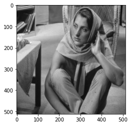
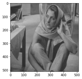
Then, import an image and show it.
# Read the image and show its size.
im = iio.imread('images/barb.tif')
print(im.shape)

# Show the image.
plt.imshow(im,cmap='gray')
These are the functions for DCT and inverse-DCT.
# Function of 2-dimensional DCT.
def dct2D(a):
    return scipy.fft.dct( scipy.fft.dct( a, axis=0, norm='ortho' ), axis=1, norm='ortho' )

# Function of 2-dimensional IDCT.
def idct2D(a):
    return scipy.fft.idct( scipy.fft.idct( a, axis=0 , norm='ortho'), axis=1 , norm='ortho')
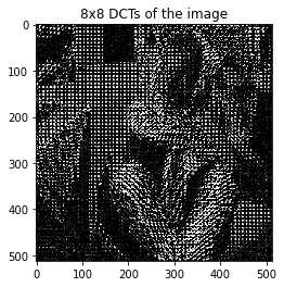
Normalize this grayscale image by subtracting 128. (The shade is represented by 0 to 255.) Then, DCT was done in an 8x8 block manner, and the DCT-ed image was shown.
# Normalize.
im = im - np.ones(im.shape)*128

# Build the array which stores DCT coeffs.
imsize = im.shape
dct = np.zeros(imsize)

# Do 8x8 DCT on image (in-place).
for i in np.arange(0, imsize[0], 8):
    for j in np.arange(0, imsize[1], 8):
        dct[i:(i+8),j:(j+8)] = dct2D( im[i:(i+8),j:(j+8)] )

# Display entire DCT.
plt.figure()
plt.imshow(dct,cmap='gray',vmax = np.max(dct)*0.01,vmin = 0)
plt.title( "8x8 DCTs of the image")
It is more convenient to deal with separated 8x8 blocks. Let’s do it!
# %% 8x8 Blocking.

# Matrix to store size-of-8x8 matrices.
dct_blocks_size = (int(imsize[0]/8),int(imsize[1]/8))
dct_blocks = np.zeros((dct_blocks_size[0],dct_blocks_size[1],8,8))

# Slice the image to size-of-8x8 matrices.
for i in np.arange(0, dct_blocks_size[0]):
    start_row = i*8
    for j in np.arange(0, dct_blocks_size[1]):
        start_col = j*8
        dct_blocks[i,j] = dct[start_row:(start_row+8),start_col:(start_col+8)]

# Display some dct blocks, with its corresponding real image blocks.
fig = plt.figure()
idx_toshow = np.array([[19,32],[23,12],[30,15]])
for idx in range(3):
    idx_row = idx_toshow[idx,0]
    idx_col = idx_toshow[idx,1]
    ax = fig.add_subplot(3, 2, idx*2+1)
    ax.imshow(im[idx_row*8:idx_row*8+8, idx_col*8:idx_col*8+8],cmap='gray')
    ax = fig.add_subplot(3, 2, idx*2+2) # this line adds sub-axes
    ax.imshow((abs(dct_blocks[idx_row,idx_col])),cmap='gray')
plt.show()
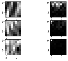
The left 8x8 blocks are from the original image, where the right 8x8 blocks are the DCT of those corresponding blocks.
Then, it’s time for quantization. The quantization table and its relation to quality are gratefully brought from seanwu1105’s prototype-jpeg repository. Hat off to him!
# %% Quantization.

def quantize(block, quality=50, inverse=False):
    quantization_table = LUMINANCE_QUANTIZATION_TABLE
    factor = 5000 / quality if quality < 50 else 200 - 2 * quality
    if inverse:
        return block * (quantization_table * factor / 100)
    return block / (quantization_table * factor / 100)

LUMINANCE_QUANTIZATION_TABLE = np.array((
    (16, 11, 10, 16, 24, 40, 51, 61),
    (12, 12, 14, 19, 26, 58, 60, 55),
    (14, 13, 16, 24, 40, 57, 69, 56),
    (14, 17, 22, 29, 51, 87, 80, 62),
    (18, 22, 37, 56, 68, 109, 103, 77),
    (24, 36, 55, 64, 81, 104, 113, 92),
    (49, 64, 78, 87, 103, 121, 120, 101),
    (72, 92, 95, 98, 112, 100, 103, 99)
))
The quantized 8x8 blocks are kept in dct_blocks_quant.
# Store quantized value in dct_block_quant.
dct_blocks_quant = np.zeros((dct_blocks_size[0],dct_blocks_size[1],8,8))
for i in np.arange(0, dct_blocks_size[0]):
    for j in np.arange(0, dct_blocks_size[1]):
        dct_blocks_quant[i,j] = quantize(dct_blocks[i,j], quality=quality)
dct_blocks_quant = np.rint(dct_blocks_quant).astype(int) # rounding to integer.

# Display some quantized dct blocks, with its corresponding dct blocks.
fig = plt.figure()
idx_toshow = np.array([[19,32],[23,12],[30,15]])
for idx in range(3):
    idx_row = idx_toshow[idx,0]
    idx_col = idx_toshow[idx,1]
    ax = fig.add_subplot(3, 2, idx*2+1)
    ax.imshow((abs(dct_blocks_quant[idx_row,idx_col])),cmap='gray')
    ax = fig.add_subplot(3, 2, idx*2+2) # this line adds sub-axes
    ax.imshow((abs(dct_blocks[idx_row,idx_col])),cmap='gray')
plt.show()
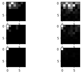
The left 8x8 blocks are from the quantized DCT blocks, where the right 8x8 blocks are the corresponding unquantized DCT blocks. You can see that further away from the DC coefficient at the upper left, the values of the AC coefficients have decreased relatively heavily.
Now, we are tempted to reconstruct the image to see how much the image has changed after the compression. Let’s begin! (Notice that it is just like stepping back from where we are.)
# %% Rescaling by quantization.

decode_dct_blocks = np.zeros((dct_blocks_size[0],dct_blocks_size[1],8,8)).astype(int)
for i in np.arange(0, dct_blocks_size[0]):
    for j in np.arange(0, dct_blocks_size[1]):
        decode_dct_blocks[i,j] = quantize(dct_blocks_quant[i,j], quality=quality, inverse=True)

# %% Reintegrating the image.

decode_dct = np.zeros((dct_blocks_size[0]*8,dct_blocks_size[1]*8))
for i in np.arange(0, dct_blocks_size[0]):
    start_row = i*8
    for j in np.arange(0, dct_blocks_size[1]):
        start_col = j*8
        decode_dct[start_row:(start_row+8),start_col:(start_col+8)] = decode_dct_blocks[i,j]

# %% Inverse DCT.

decode_im = np.zeros((dct_blocks_size[0]*8,dct_blocks_size[1]*8))
for i in np.arange(0, imsize[0], 8):
    for j in np.arange(0, imsize[1], 8):
        decode_im[i:(i+8),j:(j+8)] = idct2D( decode_dct[i:(i+8),j:(j+8)] )

# Show the image.
plt.imshow(decode_im,cmap='gray')
Reconstruction from the compressed file.
This is the way to measure PSNR.
# %% PSNR

import math

def psnr(data1, data2, max_pixel=255):
    mse = np.mean((data1 - data2) ** 2)
    if mse:
        return 20 * math.log10(max_pixel / mse ** 0.5)
    return math.inf

psnr_exp = psnr(im, decode_im)
Let’s play this code by yourself! Maybe on Google Colab, Jupyter Notebook, or Spyder. In Spyder, you can use # %% to separate a code into sections and run those one by one (just like MATLAB’s %%.) Have fun!